Activity 12: Basic Video Processing

After having to go through numerous techniques in processing images…. we are now to try and apply these to videos. Videos are known as a series of images of an event for certain time intervals. Hence, we have to find a way to convert our videos into a set of images and run our image processing techniques through loops to make things easier.

Follow the yellow brick road trail of blood

One method used in studying the rate of flow of water / liquids is through dye tracing.Some applications of dye tracing are: water flow and rate, leak detection, pollution dispersion, etc. [1].  Choosing the right type of dye for your specific study is essential as the color and type are factors on your data collection. Taking for example green dyes which are suggested to be used on murky brown waters as it gives the best contrast [1]. Taking videos of the dispersion of these dyes through the solution or samples is one of the methods in gathering data for these types of experiments.

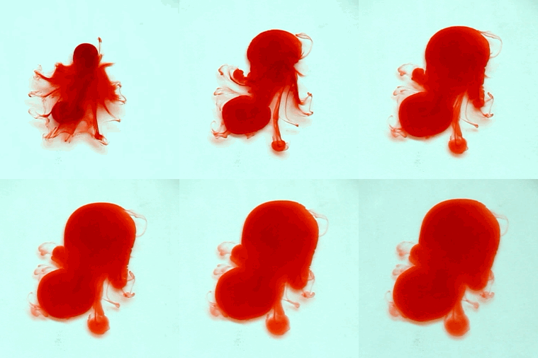
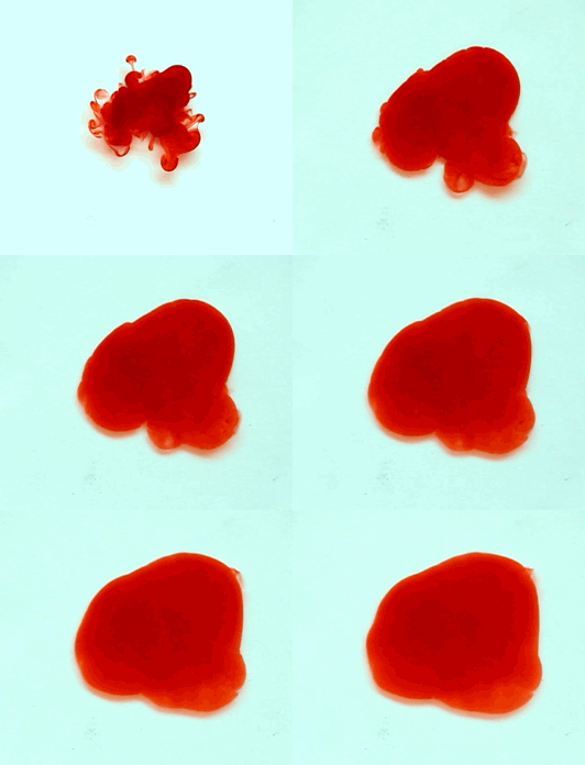
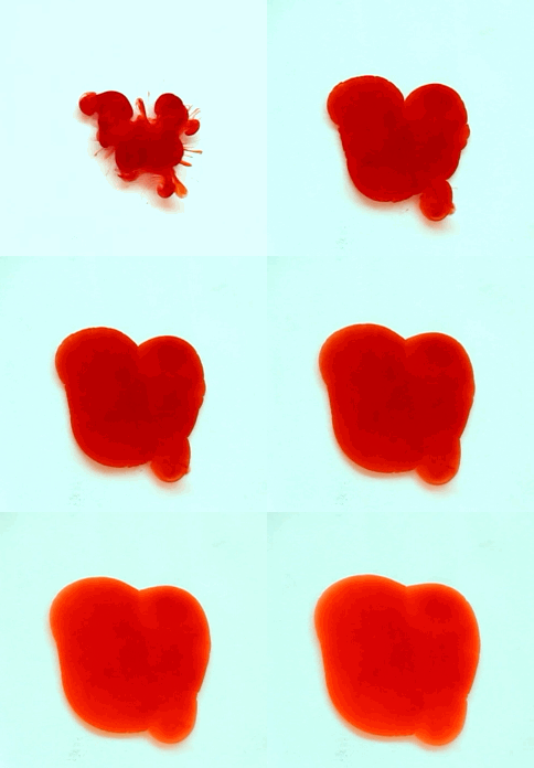
For this reason, we tried to simulate this experiment in smaller scale. A video of the dispersion of a drop of a red food coloring dye 30ml of different temperatures of water (hot, cold and tap)  placed on a petri dish was taken and this was image processed. The effect of the temperatures of the sample to the dispersion rate of a dye was investigated. A Canon EOS 550D camera was used as  the video recording device. It is known to have 50 frames per second recording ability. The video was then processed in Avidemux to be converted in a .avi file as well as for cropping off unwanted portions. The .avi file was then exported as a series of images with the ‘frames per second’ decreased to 2.5 frames per second. I was able to decrease the fps value in the program VirtualDub and this was done because making use of the typical 50fps gave me 1500 images to be processed.From visual inspection, the the change in one image to another is not that significant and hence reduction of the fps is fine just as long as the growth is observable in a smooth transition. The animations (gif) of the dispersion for the different cases below are as displayed below:

Dispersion of a red dye on a ‘cold’ water.

Dispersion of a red dye on a ‘hot’ water

Dispersion of a red dye on ‘tap’ water.

What we basically have to do is to segment our image so that we’d end up with only the dyed portions of our videos (recall Activity 11). The area of the segmented regions was then determined by simply counting the pixels having the same threshold value as the edges were not that defined as what was done before (recall Activity 4). But since we are dealing with a series of images , looping through images can be done to save time and effort (recall Activity 10).

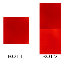
For the color segmentation portion, a region of interest (ROI) should be cropped off the image. Below are two ROI’s I have used:

The use of the 2nd ROI is necessary as after some time, the drop of dye disperses further and further resulting to a less concentrated color (lighter version). Since changing the ROI’s in a middle of a loop is complex, I instead opted to combine the lighter and darker versions. We are dealing with the mean and the standard deviation of the ROI hence ROI2 will give way into considering lighter shades as well.

Opening our images through loops is done through the use of the strcat() function. Below is the code I have used for the looping portion:

Making use of the code in Activity 11, it is not enough to simply count the pixels of a certain threshold value. The output of the segmentation resulted to pixels of differing intensity values and simply calling the maximum will give a small number(80 pixels only).  I had to make use of the code below to resolve this issue:

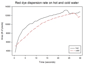
With my images sampled at a rate of 2.5 frames per second, I created a counter which would add 0.4 seconds for every image processed on my ‘time’ list. This gave me two lists (area and time) which lead me to the creation of the graphs below:

The best-fit trend was observed to be the exponential rise to a maximum as determined through the Sigmaplot plotting program. With the droplet being at its most concentrated state at the beginning, the dispersion is expected to be at its fastest rate. After some time, the  dispersion slows down as there are less and less particles pushing their way through the sample.

As for the effect of the temperature of the sample to the dispersion rate, the plot shows that there is a difference between the hot and cold water samples. It was apparent that the dispersion was faster and that the area was larger for the case of the hot water. With higher temperatures signifying faster moving particles in the sample, it is then logical that the dispersion of the dye should be faster for the hot water sample. The dye particles are also being dispersed by the particles of the water itself rather than by the dye particles colliding with one another. On the other hand, lower temperatures signify slow moving particles which gives a logical reason to the slow dispersion rate as observed from our plots.

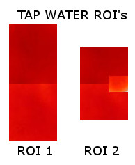
For some weird reasons, I had a hard time trying to get a nice dispersion plot for the tap water sample. With the use of the ROI2 I have used for both the hot and cold samples, I end up with a plot that suddenly decreases after some time which should not be the case! Looking at the progression of the image, the area tainted by the red dye still increases! As a solution, I had to include another cropped ROI on my current ROI as seen below:

This problem shows the need for the consistent background light for the segmentation to be a success. With the sunlight used as our light source, there will indeed be instances wherein the shades of our sample will vary.

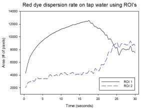
Making use of our ROI 1 and ROI 2 for our tap water sample, we end up with the plot as observed below:

The first ROI shows an exactly similar trend to that of our hot water sample for small values of t. This may indicate that the tap water temperature is still within the range where the dispersion rate is relatively fast. However, the sudden decrease in the area as detected by the ROI caused the inability to look at the rate of dispersion at later times. Making use of ROI 2 displays a different trend wherein the plot increases at an exponential trend. The sudden increases at later times shows how the values of the intensities of the pixels were much closer to our ROI (With the inclusion of the tinge of bright red)… However the downside is that at earlier times, only small amounts were segmented as the images were dominated by darker shades of red. This shows the limitations of this technique wherein the shade of the region of interest should be consistent for all times. A possible solution would be to vary the ROI’s for certain intervals so that we’d have accurate data for the area of the tainted sample.

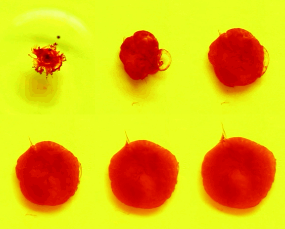
As an additional portion of our activity, we tried looking at the difference between two colored dyes. Also, we have initially added a yellow dye on our sample so that our background has its own color. Through this, we are to investigate the effectivity of the segmentation of the desired regions despite a different background color of our sample.

Red dye dispersing on a yellow tainted water medium.

Green dye dispersing on a yellow tainted water medium.

Making use of the ROI2 for our red on yellow set of images while the green on yellow images’ ROI is as presented below:

We have determined a dispersion plot showing that there is indeed a difference between the two dyes:

Again, despite having a yellow dye mixed to our water sample.. the general trend for the red dye dispersion still replicates the results from the earlier portion of this activity. The green dye on the other hands shows how it disperses at an even higher rate (as based from the slope) after a certain period of time (t = 3 seconds). This shows the difference in how the dyes react to the sample. The concentration per drop for the different colors differ hence resulting to different dispersion rates.

Note: For this activity, I was able to enjoy and at the same time learn a lot of things. Hence I would like to give myself a grade of 11/10 for getting nice results and at the same time successfully applying all the techniques I have learned throughout this course. We were also able to look at not only the effect of the temperature of the sample but also the type of dye (concentration) used. Overall, this activity was for me the most fun as it acted as a little investigatory project.

References:

1. “Guide to Dye Tracers”, Professional Equipment. Available at http://www.professionalequipment.com/guide-to-dye-tracers/articles/

PS: As much as I’d like to type in more input… the internet here in our place is crappy that I had no choice but to rush in blogging about this.. Anyway, I plan to fix this blog up even though the deadline’s over XD